Estimate yield for one species and area
Choose the forest measure, species, stand age, type of area, and area name or tile ID. The following examples estimate AGB and volume for black spruce in tile H14 at three stand ages:
predict_rsyc("agb", "PICE.MAR", c(20, 60, 120), "tile", "H14")
#> [1] 26.85001 58.32616 71.92139
predict_rsyc("volume", "PICE.MAR", c(20, 60, 120), "tile", "H14")
#> [1]  39.04578  96.87074 123.04264
The same function works for individual species and broad groups such
as coniferous and broadleaf:
species_predictions <- tibble::tibble(
  species = c("PICE.MAR", "PINU.BAN", "POPU.TRE", "coniferous", "broadleaf")
) |>
  dplyr::mutate(
    agb_80 = purrr::map_dbl(
      species,
      \(species) predict_rsyc("agb", species, 80, "tile", "H14")
    )
  )

species_predictions
#> # A tibble: 5 × 2
#>   species    agb_80
#>   <chr>       <dbl>
#> 1 PICE.MAR     65.2
#> 2 PINU.BAN     38.7
#> 3 POPU.TRE     80.9
#> 4 coniferous   52.4
#> 5 broadleaf    80.3
Multiple tiles and species
The following example estimates yield for several combinations of
forest measure, species, stand age, and tile. Each row of
tile_inputs describes one combination:
tile_inputs <- tidyr::crossing(
  response = c("agb", "volume"),
  species = c("PICE.MAR", "POPU.TRE", "coniferous"),
  age = c(20, 60, 120),
  strata_level = "tile",
  strata_id = c("H14", "F31")
) |>
  dplyr::mutate(
    prediction = purrr::pmap_dbl(
      list(response, species, age, strata_level, strata_id),
      predict_rsyc
    )
  )

tile_inputs
#> # A tibble: 36 × 6
#>    response species      age strata_level strata_id prediction
#>    <chr>    <chr>      <dbl> <chr>        <chr>          <dbl>
#>  1 agb      coniferous    20 tile         F31             41.7
#>  2 agb      coniferous    20 tile         H14             26.5
#>  3 agb      coniferous    60 tile         F31             76.3
#>  4 agb      coniferous    60 tile         H14             48.4
#>  5 agb      coniferous   120 tile         F31             87.4
#>  6 agb      coniferous   120 tile         H14             55.4
#>  7 agb      PICE.MAR      20 tile         F31             35.5
#>  8 agb      PICE.MAR      20 tile         H14             26.9
#>  9 agb      PICE.MAR      60 tile         F31             77.1
#> 10 agb      PICE.MAR      60 tile         H14             58.3
#> # ℹ 26 more rows
Before estimating many combinations, use rsyc_species()
or available_rsyc_models() to confirm that a published
curve is available for each species and tile.
Ecological areas
Use the area name when it occurs only once at the selected ecological level:
eco_inputs <- tibble::tribble(
  ~response, ~species,   ~age, ~strata_level, ~strata_id,
  "agb",     "PICE.MAR", 80,  "ecozone",
    "Atlantic Maritime",
  "agb",     "PICE.MAR", 80,  "ecoprovince",
    "Appalachian-Acadian Highlands",
  "agb",     "PICE.MAR", 80,  "ecoregion",
    "Appalachians",
  "agb",     "PICE.MAR", 80,  "ecodistrict",
    "Windsor Lowlands"
)

eco_inputs <- eco_inputs |>
  dplyr::mutate(
    prediction = purrr::pmap_dbl(
      list(response, species, age, strata_level, strata_id),
      predict_rsyc
    )
  )

eco_inputs[c("strata_level", "strata_id", "prediction")]
#> # A tibble: 4 × 3
#>   strata_level strata_id                     prediction
#>   <chr>        <chr>                              <dbl>
#> 1 ecozone      Atlantic Maritime                   71.6
#> 2 ecoprovince  Appalachian-Acadian Highlands       87.1
#> 3 ecoregion    Appalachians                        85.3
#> 4 ecodistrict  Windsor Lowlands                    50.1
Use rsyc_strata() to list area names and see where they
lie within Canada’s ecological classification. For example, more than
one ecodistrict named Salmon River has a curve for this
species and forest measure:
rsyc_strata("agb", "PICE.MAR", "ecodistrict") |>
  dplyr::filter(strata_name == "Salmon River")
#> # A tibble: 2 × 4
#>   strata_level strata_name  strata_id                                strata_code
#>   <chr>        <chr>        <chr>                                    <chr>
#> 1 ecodistrict  Salmon River Boreal Cordillera/Northern Boreal Cordi… 911
#> 2 ecodistrict  Salmon River Boreal Shield East/Newfoundland/Norther… 455

predict_rsyc(
  "agb", "PICE.MAR", 80, "ecodistrict",
  "Boreal Cordillera/Northern Boreal Cordillera/Pelly Mountains/Salmon River"
)
#> [1] 39.17884
Ecological codes can be passed through the same
strata_id argument. The selected ecological level is
required because codes can overlap between levels:
predict_rsyc(
  "agb", "PICE.MAR", 80, "ecoregion", 198
)
#> [1] 56.18245
Use quoted ecoprovince codes such as "10.1". Ecozone
codes 5, 6, and 10 are ambiguous package subdivisions, so select those
areas by name instead.
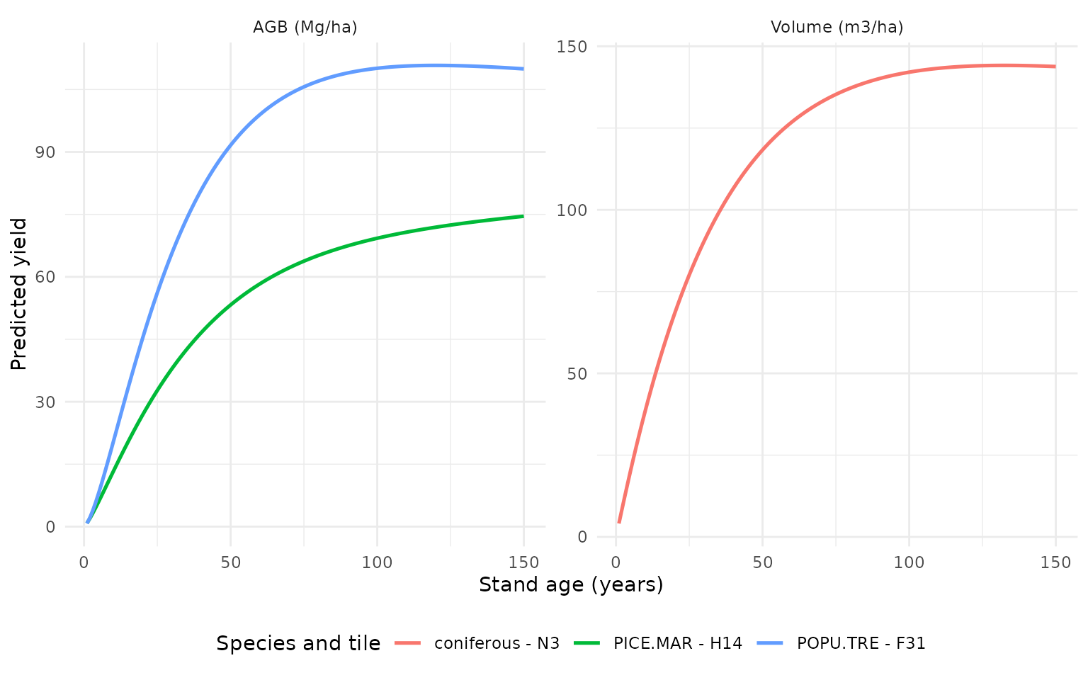
Several complete curves
This example estimates yield at ages 1 to 150 for each species and
area listed in curve_inputs:
curve_inputs <- tibble::tribble(
  ~response, ~species,     ~strata_level, ~strata_id,
  "agb",     "PICE.MAR",   "tile",       "H14",
  "agb",     "POPU.TRE",   "tile",       "F31",
  "volume",  "coniferous", "tile",       "N3"
)
curve_inputs <- curve_inputs |>
  dplyr::mutate(
    age = list(1:150),
    prediction = purrr::pmap(
      list(response, species, age, strata_level, strata_id),
      predict_rsyc
    )
  )

curve_inputs
#> # A tibble: 3 × 6
#>   response species    strata_level strata_id age         prediction
#>   <chr>    <chr>      <chr>        <chr>     <list>      <list>
#> 1 agb      PICE.MAR   tile         H14       <int [150]> <dbl [150]>
#> 2 agb      POPU.TRE   tile         F31       <int [150]> <dbl [150]>
#> 3 volume   coniferous tile         N3        <int [150]> <dbl [150]>

curve_predictions <- curve_inputs |>
  tidyr::unnest(c(age, prediction))

curve_predictions
#> # A tibble: 450 × 6
#>    response species  strata_level strata_id   age prediction
#>    <chr>    <chr>    <chr>        <chr>     <int>      <dbl>
#>  1 agb      PICE.MAR tile         H14           1      0.825
#>  2 agb      PICE.MAR tile         H14           2      1.97
#>  3 agb      PICE.MAR tile         H14           3      3.25
#>  4 agb      PICE.MAR tile         H14           4      4.60
#>  5 agb      PICE.MAR tile         H14           5      6.01
#>  6 agb      PICE.MAR tile         H14           6      7.45
#>  7 agb      PICE.MAR tile         H14           7      8.90
#>  8 agb      PICE.MAR tile         H14           8     10.4
#>  9 agb      PICE.MAR tile         H14           9     11.8
#> 10 agb      PICE.MAR tile         H14          10     13.3
#> # ℹ 440 more rows
The final table, curve_predictions, can then be plotted
or used in further analysis. AGB and volume are shown in separate panels
because they use different units:
curve_predictions |>
  dplyr::mutate(
    response = factor(
      response,
      levels = c("agb", "volume"),
      labels = c("AGB (Mg/ha)", "Volume (m3/ha)")
    ),
    curve = paste(species, strata_id, sep = " - ")
  ) |>
  ggplot2::ggplot(ggplot2::aes(age, prediction, colour = curve)) +
  ggplot2::geom_line(linewidth = 0.9) +
  ggplot2::facet_wrap(ggplot2::vars(response), scales = "free_y") +
  ggplot2::labs(
    x = "Stand age (years)",
    y = "Predicted yield",
    colour = "Species and tile"
  ) +
  ggplot2::theme_minimal() +
  ggplot2::theme(legend.position = "bottom")