Local calibration

library(RSYC)

Purpose

predict_rsyc() returns the published national curve for a given species and area. Where local field measurements are available — observed aboveground biomass (AGB) or total volume at known stand ages — calibrate_rsyc() adjusts that curve to the measured plot.

RSYC curves have a nested (hierarchical) structure: each calibration plot is treated as a pixel nested within a tile (or within an ecological unit, for curves published at an ecological level). Knowing the tile in which the calibration plot is located is therefore a prerequisite for local calibration, because the tile determines which published curve, and which tile-level random effect, the calibration starts from. Where plot coordinates are known, the tile can be identified by overlaying them on the tile boundaries returned by rsyc_boundaries("tile").

The adjustment is an empirical best linear unbiased predictor (EBLUP) of the pixel-level random effect on the curve’s asymptote parameter. Because all tiles in the target population were represented in the fitting data, the fixed asymptote parameter and the tile-level random effects were obtained directly from the fitted nonlinear mixed-effects model and are already incorporated into the published curves. Only the pixel-level random effect requires calibration. A single adjustment is estimated for the calibration plot (assumed to coincide with pixel \(j\) within tile \(i\)) and substituted into the curve equation. The estimate is shrunk toward zero in proportion to the strength of the local evidence, so a curve supported by one measurement is adjusted conservatively, whereas a curve supported by several consistent measurements is adjusted more fully.

The method

The published curve

RSYC curves were fitted as nonlinear mixed-effects models in which the tile- and pixel-level random effects act on \(\beta_1\), the parameter associated with the maximum biomass (or volume) potential of a site, referred to below as the asymptote parameter:

\[AGB_{ijk} = \left(\beta_1 + b_i + b_{ij}\right) e^{-\beta_4 age_{ijk}}\left(1 - e^{-\beta_2 age_{ijk}}\right)^{\beta_3} + \epsilon_{ijk}\]

where \(AGB_{ijk}\) is the AGB of pixel \(j\) within tile \(i\) at the \(k\)-th age \(age_{ijk}\), \(b_i\) is the random effect for tile \(i\), \(b_{ij}\) the random effect for pixel \(j\) nested within tile \(i\), and \(\epsilon_{ijk}\) the residual error. The random effects and residual errors were assumed to be independent and normally distributed with mean zero: \(b_i \sim N(0, \sigma^2_{t})\), \(b_{ij} \sim N(0, \sigma^2_b)\) and \(\epsilon_{ijk} \sim N(0, \sigma^2_\epsilon)\). The implications of this assumption are discussed under Summary and recommendations. The remaining parameters are fixed: \(\beta_2\) is the rate (scale) parameter, which determines how quickly the curve approaches its maximum, \(\beta_3\) is the shape parameter, and \(\beta_4\) controls the decline at older ages. Writing the age-related modifier separately,

\[g(age) = e^{-\beta_4 age}\left(1 - e^{-\beta_2 age}\right)^{\beta_3}\]

the curve is the maximum biomass potential multiplied by a dimensionless age-related modifier that rises from 0 toward about 1. Only \(\beta_1\) carries the random effects; \(\beta_2\), \(\beta_3\) and \(\beta_4\) are fixed, so the random effects change the magnitude of the trajectory but never its age-dependent form.

From this point onward, a hat denotes a value estimated from the fitting data (e.g. \(\hat\beta_1\), \(\hat b_i\)), and \(\hat g(age)\) denotes the age-related modifier evaluated with the estimated \(\hat\beta_2\), \(\hat\beta_3\) and \(\hat\beta_4\).

The b1 coefficient published in RSYC_models for a given tile is already the tile-level asymptote parameter \(\hat\beta_1 + \hat b_i\), not the bare population fixed effect. (parent_b1_random_effect stores \(\hat b_i\) separately for reference; it must not be added to b1.) The yield curve based on the tile-level conditional prediction, returned by predict_rsyc(), is therefore

\[\widehat{AGB}_{RSYC}(age) = \left(\hat\beta_1 + \hat b_i\right) \hat g(age) = \texttt{b1}\cdot \hat g(age)\]

Estimating the local random effect

For a calibration plot (represented by pixel \(j\) within tile \(i\)) that was not part of model fitting, the pixel-level effect \(b_{ij}\) is not available from the fitted model and must be calibrated from local observations. Because \(b_{ij}\) enters linearly through the asymptote parameter, its prediction reduces to the empirical best linear unbiased predictor (EBLUP) for a random coefficient. Given \(n_{ij}\) observations \(y_{ijk}\) at ages \(age_{ijk}\), with \(m_{ijk} = \hat g(age_{ijk})\),

\[\hat b_{ij} = \frac{\sum_{k=1}^{n_{ij}} m_{ijk}\left(y_{ijk} - \texttt{b1}\cdot m_{ijk}\right)} {\sum_{k=1}^{n_{ij}} m_{ijk}^2 + \dfrac{\hat\sigma^2_\epsilon}{\hat\sigma^2_b}}\]

where \(\hat\sigma^2_b\) is the estimated pixel-level (nested within tile) random-effect variance (local_b1_var) and \(\hat\sigma^2_\epsilon\) the estimated residual variance (residual_var) of the selected model, both estimated from the fitting sample.

Without the variance term this would be an ordinary least-squares estimate of the level shift, which would force the curve exactly through the observations. The added \(\hat\sigma^2_\epsilon/\hat\sigma^2_b\) shrinks the estimate toward zero, recognising that the observations themselves carry measurement error. The strength of that pull is summarised by the shrinkage factor

\[\lambda = \frac{\sum_k m_{ijk}^2}{\sum_k m_{ijk}^2 + \dfrac{\hat\sigma^2_\epsilon}{\hat\sigma^2_b}} \in [0, 1]\]

Values near 1 mean the local estimate is retained almost in full; values near 0 mean it is pulled back to the published curve. Because \(\hat\sigma^2_\epsilon/\hat\sigma^2_b\) is fixed by the fitted model, \(\lambda\) rises toward 1 as \(\sum_k m_{ijk}^2\) grows — with more observations, and with observations at ages where \(\hat g(age)\) is large. The formula treats the observations of a plot as independent given \(b_{ij}\), and the calibrated pixel as independent of its neighbours (see Summary and recommendations).

The calibrated curve

The estimated effect is substituted back into the asymptote parameter:

\[\widehat{AGB}^{cal}(age) = \left(\hat\beta_1 + \hat b_i + \hat b_{ij}\right) \hat g(age) = \left(\texttt{b1} + \hat b_{ij}\right) \hat g(age)\]

Equivalently, this scales the published curve by the age-independent ratio \((\texttt{b1} + \hat b_{ij})/\texttt{b1}\), reported as ratio_blup (with \(\hat b_{ij}\) reported as b_pixel). The two statements are the same operation written differently, since \(\hat g(age)\) cancels.

Example 1: a single observation

A single measurement is sufficient to calibrate \(\hat b_{ij}\), although the weight it receives depends on the age at which it was taken (see How shrinkage depends on age). In this example a black spruce plot in tile H14 was measured once, at age 60:

single <- calibrate_rsyc(
  response = "agb",
  species = "PICE.MAR",
  strata_level = "tile",
  strata_id = "H14",
  obs_age = 60,
  obs_response = 83.8
)

single$shrinkage_factor
#> [1] 0.8777606
single$b_pixel
#> [1] 26.15953
single$ratio_blup
#> [1] 1.38336

The estimated adjustment to the asymptote parameter, \(\hat b_{ij}\), is 26.2 Mg/ha, corresponding to a ratio of 1.38, an increase of approximately 38% relative to the published curve. None of the constraints described below were reached:

c(
  random_effect = single$random_effect_limited,
  ratio = single$ratio_limited,
  value = single$value_limited
)
#> random_effect         ratio         value 
#>         FALSE         FALSE         FALSE

Evaluating the calibrated curve over the full age range shows the published and calibrated curves running parallel, separated by the constant ratio:

single_curve <- calibrate_rsyc(
  "agb", "PICE.MAR", "tile", "H14",
  obs_age = 60, obs_response = 83.8,
  predict_age = 1:150
)

single_long <- tidyr::pivot_longer(
  single_curve$predictions,
  c(value, value_uncalibrated),
  names_to = "series", values_to = "agb"
)
single_long$series <- factor(
  single_long$series,
  levels = c("value_uncalibrated", "value"),
  labels = c("Published curve", "Calibrated curve")
)

ggplot2::ggplot(single_long, ggplot2::aes(age, agb, colour = series)) +
  ggplot2::geom_line(linewidth = 0.9) +
  ggplot2::geom_point(
    data = tibble::tibble(age = 60, agb = 83.8),
    ggplot2::aes(age, agb), inherit.aes = FALSE, size = 3
  ) +
  ggplot2::labs(
    x = "Stand age (years)", y = "AGB (Mg/ha)", colour = NULL,
    title = "Single-observation calibration, black spruce, tile H14"
  ) +
  ggplot2::theme_minimal() +
  ggplot2::theme(legend.position = "bottom")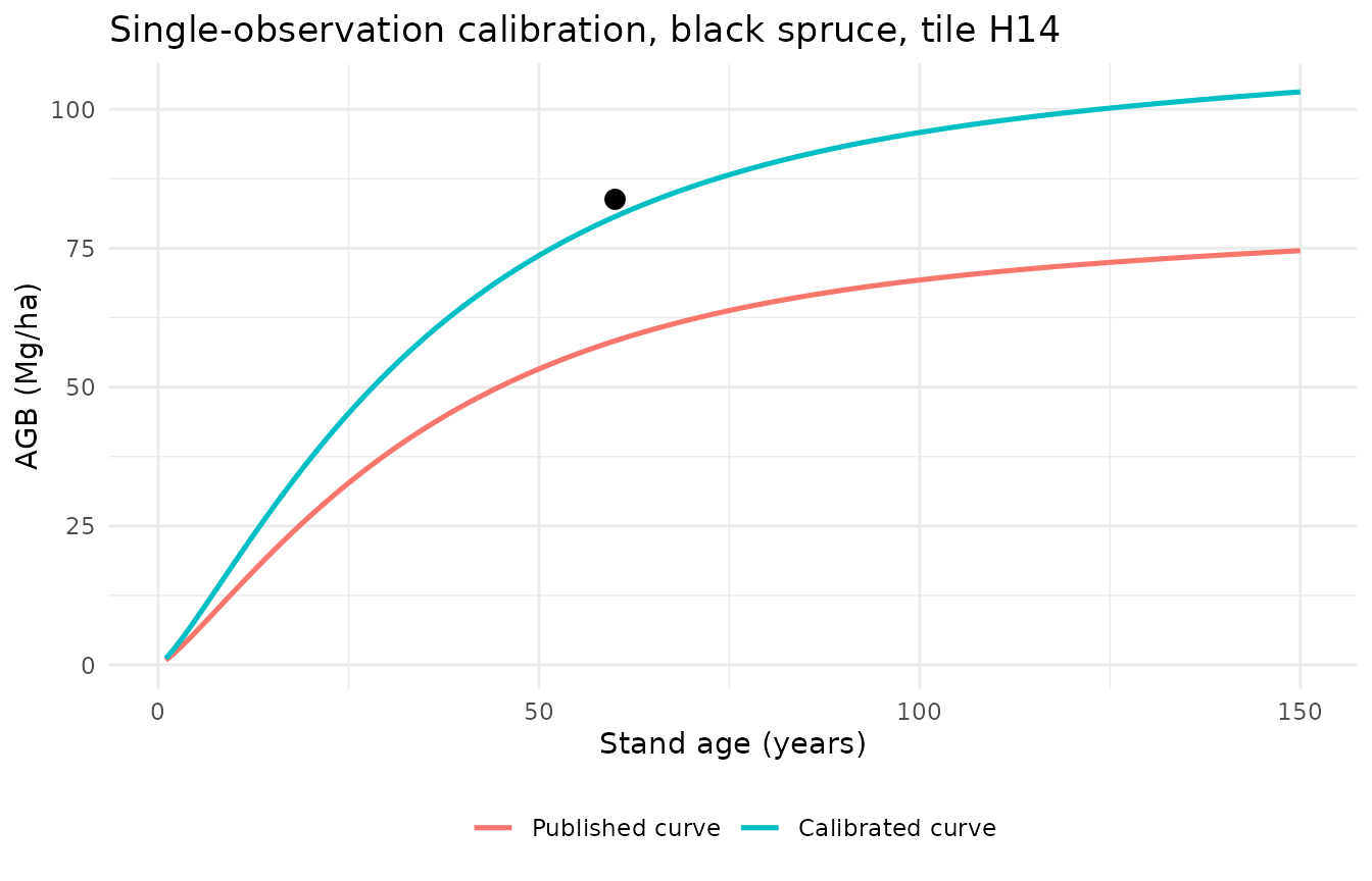

With one measurement the result is best described as a single-observation BLUP-anchored curve: it re-levels the published curve, but it does not learn a new growth trajectory from one point.

Example 2: several observations

Repeated measurements of the same stand provide more evidence, so the estimate is shrunk less. The observations below are scattered on either side of the fitted trajectory, as repeated field measurements typically are:

multiple <- calibrate_rsyc(
  "agb", "PICE.MAR", "tile", "H14",
  obs_age = c(32, 48, 61, 77, 94),
  obs_response = c(54.6, 58.6, 76.7, 72.0, 86.8)
)

tibble::tibble(
  case = c("single observation", "five observations"),
  n_obs = c(single$n_obs, multiple$n_obs),
  shrinkage_factor = c(single$shrinkage_factor, multiple$shrinkage_factor),
  b_pixel = c(single$b_pixel, multiple$b_pixel),
  ratio_blup = c(single$ratio_blup, multiple$ratio_blup)
)
#> # A tibble: 2 × 5
#>   case               n_obs shrinkage_factor b_pixel ratio_blup
#>   <chr>              <int>            <dbl>   <dbl>      <dbl>
#> 1 single observation     1            0.878    26.2       1.38
#> 2 five observations      5            0.972    15.0       1.22

The shrinkage factor increases from 0.88 to 0.97, so a greater proportion of the estimated departure from the published curve is retained.

multi_curve <- calibrate_rsyc(
  "agb", "PICE.MAR", "tile", "H14",
  obs_age = c(32, 48, 61, 77, 94),
  obs_response = c(54.6, 58.6, 76.7, 72.0, 86.8),
  predict_age = 1:150
)

multi_long <- tidyr::pivot_longer(
  multi_curve$predictions,
  c(value, value_uncalibrated),
  names_to = "series", values_to = "agb"
)
multi_long$series <- factor(
  multi_long$series,
  levels = c("value_uncalibrated", "value"),
  labels = c("Published curve", "Calibrated curve")
)

ggplot2::ggplot(multi_long, ggplot2::aes(age, agb, colour = series)) +
  ggplot2::geom_line(linewidth = 0.9) +
  ggplot2::geom_point(
    data = tibble::tibble(
      age = c(32, 48, 61, 77, 94),
      agb = c(54.6, 58.6, 76.7, 72.0, 86.8)
    ),
    ggplot2::aes(age, agb), inherit.aes = FALSE, size = 2.5
  ) +
  ggplot2::labs(
    x = "Stand age (years)", y = "AGB (Mg/ha)", colour = NULL,
    title = "Calibration from five observations, black spruce, tile H14"
  ) +
  ggplot2::theme_minimal() +
  ggplot2::theme(legend.position = "bottom")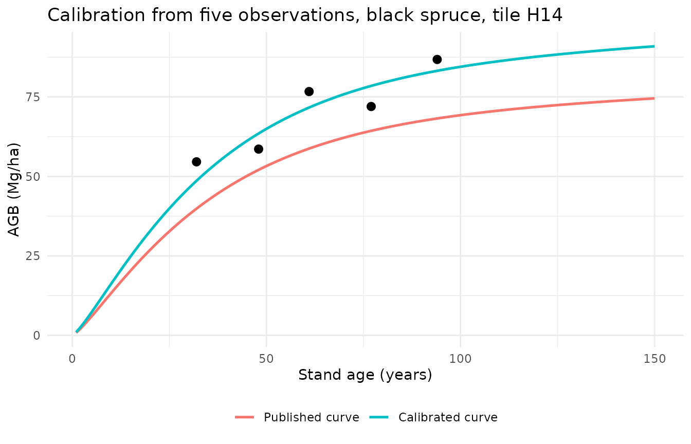

The calibrated curve passes among the observations rather than through them, and retains the shape of the published curve. Both properties follow from the method: only the asymptote parameter is adjusted, and that adjustment is shrunk by \(\lambda\). Here \(\lambda \approx 0.97\), so approximately 97% of the estimated departure is retained. The remainder reflects the model attributing part of the discrepancy to residual error rather than to a genuine difference in site productivity. An ordinary least-squares fit would reproduce the observations exactly, but would also propagate their measurement error to predictions at all other ages.

How shrinkage depends on age

Because \(\lambda\) depends on \(\sum_k m_{ijk}^2\), a single observation does not always carry the same weight. A measurement in a young stand sits low on the age-related modifier (\(\hat g(age) \approx 0\)) and says little about the maximum biomass potential, so it is shrunk heavily. A measurement in a mature stand is trusted far more:

model <- subset(
  RSYC_models,
  response == "agb" & scale == "national" &
    strata_level == "tile" & strata_id == "H14" & species == "PICE.MAR"
)
variance_ratio <- model$residual_var[[1L]] / model$local_b1_var[[1L]]

modifier <- exp(-model$b4[[1L]] * (1:150)) *
  (1 - exp(-model$b2[[1L]] * (1:150)))^model$b3[[1L]]

shrinkage_by_age <- tibble::tibble(
  age = 1:150,
  shrinkage_factor = modifier^2 / (modifier^2 + variance_ratio)
)

ggplot2::ggplot(
  shrinkage_by_age, ggplot2::aes(age, shrinkage_factor)
) +
  ggplot2::geom_line(linewidth = 0.9) +
  ggplot2::ylim(0, 1) +
  ggplot2::labs(
    x = "Age of the single observation (years)",
    y = expression(paste("Shrinkage factor ", lambda)),
    title = "Informativeness of a single observation by stand age"
  ) +
  ggplot2::theme_minimal()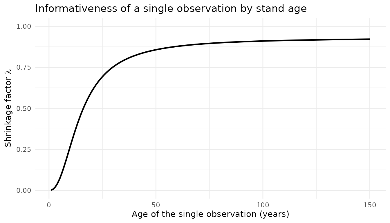

For this model, the shrinkage factor of a single observation is 0.27 at age 10, 0.86 at age 50 and 0.91 at age 100: it rises steeply in young stands and changes little after about age 50. A young stand has not yet expressed much of its eventual productivity potential, so a single young-age measurement provides little information about the asymptote parameter and the EBLUP is shrunk strongly toward zero. In older stands the development trajectory is more predictable; the same reasoning underlies the common use of an index age of 50 years for site index in Canada.

Consequently the number of observations alone does not determine the weight given to local data: several measurements in young stands may be less informative about the asymptote parameter than one measurement in a mature stand. When collecting data for calibration, plots in stands that have already expressed much of their productivity potential (e.g. older than about 50 years) should be preferred.

Calibrating volume across several stands

The same procedure applies to total volume. The example below calibrates four independent stands, each with three measurements, using ecoregion-level models for four species. Each stand is calibrated separately against its own model:

field_plots <- tibble::tribble(
  ~plot, ~species,   ~ecoregion,                 ~age,          ~volume,
  "A",   "PICE.MAR", "Appalachians",             c(45, 62, 80), c(135.8, 165.7, 172.7),
  "B",   "POPU.TRE", "Saint John River Valley",  c(30, 44, 58), c(100.5, 150.7, 172.8),
  "C",   "PICE.GLA", "Annapolis-Minas Lowlands", c(55, 70, 88), c(110.9, 121.1, 112.5),
  "D",   "PINU.BAN", "Boreal Plains/Central Boreal Plains/Mid-Boreal Uplands",
                                                 c(38, 52, 66), c(62.9, 65.4, 85.0)
)

calibrations <- purrr::pmap(
  list(field_plots$species, field_plots$ecoregion,
       field_plots$age, field_plots$volume),
  \(species, ecoregion, age, volume) {
    calibrate_rsyc(
      "volume", species, "ecoregion", ecoregion,
      obs_age = age, obs_response = volume
    )
  }
)

field_plots |>
  dplyr::mutate(
    n_obs = purrr::map_int(calibrations, "n_obs"),
    shrinkage_factor = purrr::map_dbl(calibrations, "shrinkage_factor"),
    ratio_blup = purrr::map_dbl(calibrations, "ratio_blup")
  ) |>
  dplyr::select(plot, species, n_obs, shrinkage_factor, ratio_blup)
#> # A tibble: 4 × 5
#>   plot  species  n_obs shrinkage_factor ratio_blup
#>   <chr> <chr>    <int>            <dbl>      <dbl>
#> 1 A     PICE.MAR     3            0.955      1.18 
#> 2 B     POPU.TRE     3            0.960      0.926
#> 3 C     PICE.GLA     3            0.974      1.10 
#> 4 D     PINU.BAN     3            0.938      0.961

Ratios below 1 indicate stands less productive than the published curve for their species and ecoregion, and ratios above 1 indicate more productive stands. Note that Mid-Boreal Uplands occurs in more than one ecozone, so the full hierarchical path is required to identify it; rsyc_strata() lists the available names and paths.

plot_curves <- purrr::pmap(
  list(field_plots$plot, field_plots$species, field_plots$ecoregion),
  \(plot, species, ecoregion) {
    fit <- calibrate_rsyc(
      "volume", species, "ecoregion", ecoregion,
      obs_age = field_plots$age[[which(field_plots$plot == plot)]],
      obs_response = field_plots$volume[[which(field_plots$plot == plot)]],
      predict_age = 1:150
    )
    fit$predictions |>
      dplyr::mutate(plot = plot, species = species)
  }
) |>
  dplyr::bind_rows() |>
  tidyr::pivot_longer(
    c(value, value_uncalibrated),
    names_to = "series", values_to = "volume"
  ) |>
  dplyr::mutate(
    series = factor(
      series,
      levels = c("value_uncalibrated", "value"),
      labels = c("Published curve", "Calibrated curve")
    )
  )

plot_points <- field_plots |>
  tidyr::unnest(c(age, volume)) |>
  dplyr::select(plot, species, age, volume)

ggplot2::ggplot(plot_curves, ggplot2::aes(age, volume, colour = series)) +
  ggplot2::geom_line(linewidth = 0.8) +
  ggplot2::geom_point(
    data = plot_points, ggplot2::aes(age, volume),
    inherit.aes = FALSE, size = 2
  ) +
  ggplot2::facet_wrap(
    ggplot2::vars(paste0(plot, ": ", species)), scales = "free_y"
  ) +
  ggplot2::labs(
    x = "Stand age (years)", y = expression(Volume~(m^3~ha^-1)),
    colour = NULL
  ) +
  ggplot2::theme_minimal() +
  ggplot2::theme(legend.position = "bottom")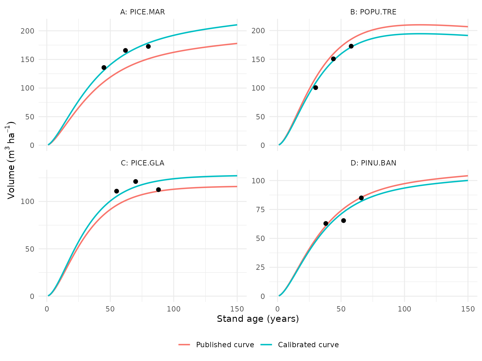

Constraints on the adjustment

By default (apply_limits = TRUE) three constraints prevent implausible adjustments arising from extreme or sparse observations:

• the local effect \(\hat b_{ij}\) is constrained to \(\pm\)random_effect_limit_sd \(\times\,\hat\sigma_b\), which at the default of 3 corresponds to the central 99.7% of the fitted pixel-level random-effect distribution;
• an adjustment ratio exceeding ratio_limit is discarded, and the published curve is returned unchanged;
• any calibrated value exceeding value_limit reverts to the published curve.

Each constraint sets a corresponding flag when it takes effect, so its influence can be quantified across a set of stands. None of the examples above required any of them. Imposing a deliberately restrictive ratio_limit demonstrates the behaviour:

constrained <- calibrate_rsyc(
  "agb", "PICE.MAR", "tile", "H14",
  obs_age = 60, obs_response = 83.8,
  ratio_limit = 1.05
)

constrained$ratio_limited
#> [1] TRUE
constrained$ratio_blup
#> [1] 1

Setting apply_limits = FALSE returns the unconstrained shrunk estimate. This is useful when quantifying how often the constraints are reached, but it removes the protection against unstable local fits, so the defaults are recommended for routine use.

Summary and recommendations

Local calibration requires:

• the tile (or ecological unit) in which the calibration plot is located, usually derived from the plot’s XY coordinates and rsyc_boundaries();
• the species and response ("agb" or "volume");
• one or more local measurements with the corresponding stand ages;
• the model parameters and variance components (\(\texttt{b1}\), \(\hat\beta_2\), \(\hat\beta_3\), \(\hat\beta_4\), \(\hat\sigma^2_b\), \(\hat\sigma^2_\epsilon\)), which calibrate_rsyc() takes automatically from RSYC_models.

Calibration works best with repeated measurements of the same plot and with measurements taken at or after about age 50, when the stand has expressed much of its productivity potential. The default constraints should normally be kept.

Several limitations should be kept in mind:

• Calibration adjusts only the asymptote parameter. It re-levels the published curve but cannot change its age-dependent form.
• The pixel-level random effects were assumed to be independent. This was reasonable for model fitting, because the fitting sample was spaced 500 m apart, but neighbouring pixels are likely to be spatially autocorrelated. The model therefore provides no basis for transferring a calibration from the measured plot to adjacent pixels, and it does not represent local (microsite) variation in productivity within a stand.
• Predictions for an individual pixel or plot are consequently the least reliable. Because forest management decisions are usually made at stand or landscape scales, predictions aggregated to those scales are likely to be more reliable.